
Executive Summary
The purpose of this document is to teach a learner who has finished "Building an AI Draughts Game for the Web" the core ideas of machine learning, by making the game's computer opponent learn from games it plays against itself. The course replaces the hand-written rule that scores positions, first with numbers tuned by self-play in the way Arthur Samuel described in 1959, then with a small neural network written from first principles in Python and run inside the existing search in the browser. The scope covers parameters, fair matches between programs, hill climbing, the statistics needed to judge an improvement, how a neural network learns, training data, overfitting, and deployment. Large models, graphics cards and machine-learning frameworks are deliberately out of scope.
Every script in this course was run before the course was written, and every result quoted comes from those runs, with fixed random seeds so that learners can reproduce them. Each learned evaluation was judged by playing hundreds of games against the hand-written rule from Course 1 at the same search depth, on openings never used in training, and reporting the score with a 95% range. The matters assessed are whether self-play tuning, a neural network on its own, and a combination of the hand-written rule with a network each play measurably better than the original. Sources are listed in the appendix.
Module 0: Before You Start
What you will build
In Course 1 the computer opponent searched ahead with minimax and judged each position with a rule of thumb you wrote by hand: a man is worth 100 points, a king 175, and so on. In this course the computer learns its own judgement by playing itself, in two ways.
Learned numbers. Keep the same rule, but let the computer adjust its numbers, keeping each change only if it wins more games
A neural network. Replace the rule with a small network that has looked at hundreds of thousands of positions and learned which ones tend to be won
You will add two new strengths to the game, Learned and Neural, and, more importantly, you will measure honestly whether either is really better.
Teacher's note: This course reports real results, including the disappointing ones. Machine learning does not always work first time, and learning to tell a real improvement from a lucky one is the most valuable skill in the course.
What you need
The finished Course 1 project
Node.js, as used for the tests in Course 1
NumPy, a Python package for working with large tables of numbers
Make a copy of your Course 1 folder called draughts-learn and open it in VS Code.
Your copy includes the venv folder, but a virtual environment cannot be copied: the copy still points at the folder where it was first made, so anything you install would go there instead. In the copy, delete the venv folder, then create and activate a new one exactly as in Course 1, and install the packages with pip install -r requirements.txt.
Teacher's note: On a Mac, AirPlay Receiver uses port 5000, the port the game uses when you run python app.py on your computer. If Flask says the port is already in use, or the browser shows an error instead of the game, turn AirPlay Receiver off (on macOS 13 or later in System Settings, General, AirDrop and Handoff; on macOS 12 in System Preferences, Sharing), or change port=5000 to port=5001 in the last line of app.py and open http://127.0.0.1:5001 instead.
Next, create a folder called train, and inside it a folder called data. Then create train/requirements.txt containing the single word numpy, and install it into the new virtual environment.
pip install -r train/requirements.txtNumPy is only needed on your own computer, for training. The server never trains anything, so it does not need NumPy.
How long things take
On the computer used to write this course, the slowest step, the final comparison at search depth 4, took about five minutes. Self-play took about 80 seconds, hill climbing about a minute and training the network about 15 seconds. Your computer may be faster or slower.
Module 1: From Rules of Thumb to Parameters
Numbers that can change
Look again at the evaluation function from Course 1. It contains five numbers that someone chose by hand: 100 for a man, 175 for a king, 3 for each row a man has advanced, 6 for a man guarding its back row, and 4 for a piece in the centre. A number inside a program that could be set differently is called a parameter. Machine learning is, at heart, the business of setting parameters from data or experience instead of by hand.
The new ai.js
The search stays exactly as it was in Course 1. What changes is that the evaluation function can now be swapped, and its numbers passed in.
WEIGHTSgathers the five hand-written numbers in one placeevaluateWithis the Course 1 rule, but it takes its numbers as an argumentevaluatorForpicks an evaluation by name:hand,learned,neural,hybrid, orcustomwith numbers supplied by a training scriptchooseMovenow accepts either a level name or a settings object, and an optional random number generator so that experiments can be repeated exactly
Replace static/js/ai.js with the version below. It refers to two files you will create later, learned-weights.js and nn.js; Module 3 and Module 6 explain them. Until you create them for real, make two placeholder files so the game still loads, as described at the end of this module.
File: static/js/ai.js
/*
 * ai.js - the computer opponent.
 *
 * The AI uses MINIMAX search with ALPHA-BETA PRUNING (see Course 1). What is
 * new in Course 3 is that the EVALUATION FUNCTION - the rule of thumb that
 * scores a position at the end of the search - can now be swapped:
 *
 *   'hand'    the hand-written rule from Course 1, using the numbers in WEIGHTS
 *   'learned' the same rule, using numbers found by self-play (learned-weights.js)
 *   'neural'  a small neural network trained on self-play games (nn.js)
 *   'hybrid'  the hand-written rule plus a correction from the network
 *
 * The search itself never changes. That lets us compare evaluation functions
 * fairly: same search, same depth, different judgement.
 */

// In the browser these are globals; in Node we load them.
const RulesLib = (typeof Rules !== 'undefined') ? Rules : require('./rules.js');
const Learned = (typeof LEARNED_WEIGHTS !== 'undefined') ? LEARNED_WEIGHTS
  : require('./learned-weights.js');
const Neural = (typeof NeuralEval !== 'undefined') ? NeuralEval : require('./nn.js');

const AI = (function () {
  // The hand-written numbers from Course 1, now gathered in one place.
  const WEIGHTS = { man: 100, king: 175, advance: 3, backRow: 6, centre: 4 };

  const LEVELS = {
    easy:    { depth: 2, randomChance: 0.35, evaluator: 'hand' },
    medium:  { depth: 4, randomChance: 0.10, evaluator: 'hand' },
    hard:    { depth: 7, randomChance: 0,    evaluator: 'hand' },
    learned: { depth: 7, randomChance: 0,    evaluator: 'learned' },
    neural:  { depth: 5, randomChance: 0,    evaluator: 'hybrid' }
  };

  const WIN_SCORE = 100000;
  const HYBRID_SCALE = 300;

  /*
   * The hand-written evaluation, with its numbers passed in as `w`.
   * Positive = good for `player`, negative = good for the opponent.
   */
  function evaluateWith(w, board, player) {
    let score = 0;
    for (let r = 0; r < 8; r++) {
      for (let c = 0; c < 8; c++) {
        const p = board[r][c];
        if (p === '.') continue;
        let value;
        if (RulesLib.isKing(p)) {
          value = w.king;
        } else {
          const advance = (p === 'b') ? (7 - r) : r;
          value = w.man + advance * w.advance;
          if ((p === 'b' && r === 7) || (p === 'w' && r === 0)) value += w.backRow;
        }
        if (r >= 2 && r <= 5 && c >= 2 && c <= 5) value += w.centre;
        score += RulesLib.ownerOf(p) === player ? value : -value;
      }
    }
    return Math.round(score);
  }

  // Pick the evaluation function by name. Each returns a whole number.
  function evaluatorFor(name, weights) {
    if (name === 'learned') return (b, p) => evaluateWith(Learned, b, p);
    if (name === 'neural') return (b, p) => Neural.evaluate(b, p);
    // Hybrid: keep the hand-written knowledge and let the network adjust it.
    // HYBRID_SCALE says how much the network's opinion counts (300 is about
    // three men). It was a first guess; tuning it is an exercise in the course.
    if (name === 'hybrid') {
      return (b, p) => evaluateWith(WEIGHTS, b, p) + Math.round(HYBRID_SCALE * Neural.predict(b, p));
    }
    if (name === 'custom') return (b, p) => evaluateWith(weights, b, p);
    return (b, p) => evaluateWith(WEIGHTS, b, p);
  }

  // Minimax with alpha-beta pruning, exactly as in Course 1, except that the
  // evaluation function arrives in `ctx` instead of being fixed.
  function minimax(state, depth, alpha, beta, maximising, ctx) {
    ctx.nodes++;
    const moves = RulesLib.legalMoves(state);
    if (moves.length === 0) return maximising ? -WIN_SCORE - depth : WIN_SCORE + depth;
    if (depth === 0) return ctx.evaluate(state.board, ctx.player);

    let best = maximising ? -Infinity : Infinity;
    for (const move of moves) {
      const score = minimax(RulesLib.applyMove(state, move), depth - 1, alpha, beta, !maximising, ctx);
      if (maximising) {
        best = Math.max(best, score);
        alpha = Math.max(alpha, best);
      } else {
        best = Math.min(best, score);
        beta = Math.min(beta, best);
      }
      if (alpha >= beta) break;
    }
    return best;
  }

  /*
   * Choose a move. `level` is a name from LEVELS, or a settings object such as
   * { depth: 3, randomChance: 0, evaluator: 'custom', weights: {...} }
   * which the training scripts use. `rand` lets scripts supply a seeded
   * random number generator so experiments can be repeated exactly.
   */
  function chooseMove(state, level, rand = Math.random) {
    const settings = typeof level === 'string' ? (LEVELS[level] || LEVELS.medium) : level;
    const moves = RulesLib.legalMoves(state);
    if (moves.length === 0) return null;
    if (moves.length === 1) return moves[0];
    if (rand() < settings.randomChance) return moves[Math.floor(rand() * moves.length)];

    const ctx = { player: state.turn, nodes: 0,
                  evaluate: evaluatorFor(settings.evaluator, settings.weights) };
    let bestScore = -Infinity;
    let bestMoves = [];
    for (const move of moves) {
      const score = minimax(RulesLib.applyMove(state, move), settings.depth - 1,
                            bestScore - 1, Infinity, false, ctx);
      if (score > bestScore) { bestScore = score; bestMoves = [move]; }
      else if (score === bestScore) bestMoves.push(move);
    }
    return bestMoves[Math.floor(rand() * bestMoves.length)];
  }

  return { WEIGHTS, LEVELS, WIN_SCORE, evaluateWith, chooseMove };
})();

if (typeof module !== 'undefined') module.exports = AI;
Keeping the search fixed and changing only the evaluation is the key to fair experiments. If a learned evaluation wins more games, the only possible reason is its judgement of positions.
Placeholder files
Create static/js/learned-weights.js with the hand-written numbers, so the Learned level starts out identical to High.
const LEARNED_WEIGHTS = { man: 100, king: 175, advance: 3, backRow: 6, centre: 4 };
if (typeof module !== 'undefined') module.exports = LEARNED_WEIGHTS;
You will create nn.js in Module 6 and train nn-weights.js in Module 7. If you want to test the game before then, leave the Neural option out of index.html until Module 8.
Check your progress
node tests/test_rules.js still passes all 8 Course 1 tests, which shows the search behaves as before.
Module 2: Fair Matches Between Programs
Why a match needs care
To find out whether one evaluation is better than another, we let them play each other many times. Three problems have to be solved first.
Variety. Two programs that always choose the same move would play the same game every time. So each game starts from a short random opening of four to eight moves
Fairness. Some openings favour one side, and moving first may matter. So every opening is played twice, with the colours swapped
Repeatability. Random openings would make every run different. So the randomness comes from a seeded random number generator: given the same seed, it produces the same sequence of numbers every time
Measuring the result
Each game scores 1 for a win, a half for a draw and 0 for a loss, and the score is the average. A score of 50% means "no better and no worse".
No match is long enough to remove luck completely, so the result comes with a 95% range: the band in which we would expect the true score to lie, 95 times in 100. We work it out from the standard error, which measures how much a score would wobble from match to match.
standard error = square root of ( score x (1 - score) / games )
95% range      = score minus 1.96 standard errors, to score plus 1.96 standard errors
This is an approximation, and it slightly overstates the wobble when there are many draws, which errs on the side of caution. The rule to remember is simple: if the 95% range includes 50%, the match has not shown a difference.
The listing
Create train/match.js.
File: train/match.js
/*
 * train/match.js - play matches between two AI settings and report the result.
 *
 * Used by every experiment in Course 3. A fair match needs three things:
 *   1. Variety. Two deterministic programs would play the same game every
 *      time, so each game starts from a short random opening.
 *   2. Fairness. Each opening is played twice, with the colours swapped,
 *      so neither side gains from a lucky opening or from moving first.
 *   3. Honesty about chance. The result comes with a 95% range, so we can
 *      tell a real improvement from a lucky run.
 */

const Rules = require('../static/js/rules.js');
const AI = require('../static/js/ai.js');

// A small random number generator with a seed ("mulberry32"), so every
// experiment can be repeated exactly.
function seeded(seed) {
  return function () {
    seed |= 0; seed = seed + 0x6D2B79F5 | 0;
    let t = Math.imul(seed ^ seed >>> 15, 1 | seed);
    t = t + Math.imul(t ^ t >>> 7, 61 | t) ^ t;
    return ((t ^ t >>> 14) >>> 0) / 4294967296;
  };
}

// Play a few random legal moves to reach a varied starting position.
function randomOpening(rand, minPlies = 4, maxPlies = 8) {
  let state = Rules.newGame();
  const plies = minPlies + Math.floor(rand() * (maxPlies - minPlies + 1));
  for (let i = 0; i < plies && !Rules.result(state); i++) {
    const moves = Rules.legalMoves(state);
    state = Rules.applyMove(state, moves[Math.floor(rand() * moves.length)]);
  }
  return state;
}

// Play one game. Returns 'b', 'w' or 'draw'. Very long games count as draws.
function playGame(start, black, white, rand, maxPlies = 200, onPosition = null) {
  let state = start;
  for (let ply = 0; ply < maxPlies; ply++) {
    const outcome = Rules.result(state);
    if (outcome) return outcome.winner;
    if (onPosition) onPosition(state);
    const settings = state.turn === 'b' ? black : white;
    state = Rules.applyMove(state, AI.chooseMove(state, settings, rand));
  }
  return 'draw';
}

/*
 * Play `pairs` openings, each twice with colours swapped, between settings
 * A and B. Returns A's results. Score = (wins + half the draws) / games.
 */
function match(a, b, pairs, seed) {
  const rand = seeded(seed);
  let wins = 0, draws = 0, losses = 0;
  for (let i = 0; i < pairs; i++) {
    const start = randomOpening(rand);
    for (const aIsBlack of [true, false]) {
      const winner = aIsBlack ? playGame(start, a, b, rand) : playGame(start, b, a, rand);
      const aColour = aIsBlack ? 'b' : 'w';
      if (winner === 'draw') draws++;
      else if (winner === aColour) wins++;
      else losses++;
    }
  }
  const games = wins + draws + losses;
  const score = (wins + draws / 2) / games;
  // 95% range using the normal approximation: score +/- 1.96 standard errors.
  const se = Math.sqrt(score * (1 - score) / games);
  return { games, wins, draws, losses, score,
           low: Math.max(0, score - 1.96 * se), high: Math.min(1, score + 1.96 * se) };
}

function describe(r) {
  const pct = x => (100 * x).toFixed(1) + '%';
  return `${r.games} games: ${r.wins} won, ${r.draws} drawn, ${r.losses} lost. ` +
         `Score ${pct(r.score)} (95% range ${pct(r.low)} to ${pct(r.high)})`;
}

module.exports = { seeded, randomOpening, playGame, match, describe };
Check your progress
Type node -e "const M=require('./train/match.js'); const h={depth:3,randomChance:0,evaluator:'hand'}; console.log(M.describe(M.match(h,h,10,1)))". Two identical players should score close to 50%, with a range that includes 50%.
Module 3: Hill Climbing, as Samuel Did in 1959
The idea
In 1959 Arthur Samuel of IBM published a paper describing a checkers program that improved its own scoring rule by playing against a copy of itself. One version adjusted its numbers; whenever it won, the other version copied them. Our version is the simplest form of that idea, called hill climbing: make a small change, keep it if it helps, and repeat. Imagine climbing a hill in fog by always stepping in whichever direction goes up.
Figure 1 shows the steps.
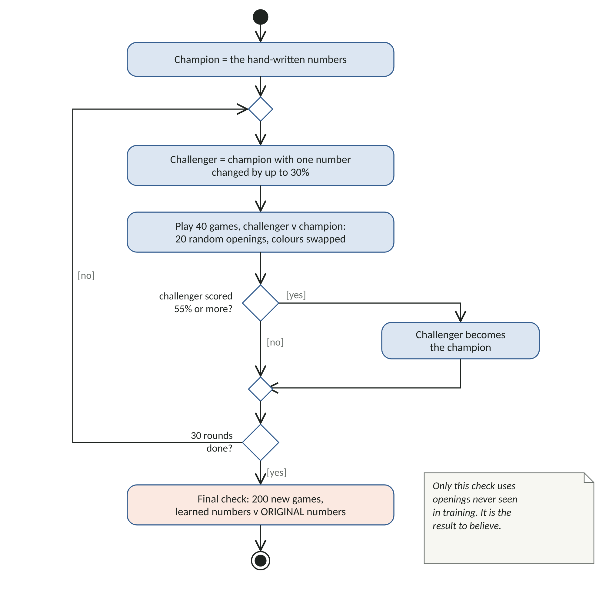
Figure 1: UML activity diagram of hill climbing by self-play.
Three choices in the script are worth noticing.
The value of a man stays fixed at 100. It acts as the unit that everything else is measured in, so the other numbers have something to be compared against
Training uses a search depth of 3, so that each round of 40 games takes only a couple of seconds
A challenger must score at least 55% to replace the champion
The listing
Create train/hillclimb.js. At the end it writes the learned numbers into static/js/learned-weights.js, replacing your placeholder.
File: train/hillclimb.js
/*
 * train/hillclimb.js - learn better numbers for the evaluation by self-play.
 *
 * This is the idea Arthur Samuel used for checkers in 1959, in its simplest form:
 *   1. Start with the hand-written numbers (the "champion").
 *   2. Make a small random change to one number (the "challenger").
 *   3. Let the challenger play the champion. If it scores well enough, it
 *      becomes the new champion.
 *   4. Repeat.
 * At the end, a separate, larger match against the ORIGINAL numbers tells us
 * whether the learning really helped - or whether we were fooled by luck.
 *
 * Run:  node train/hillclimb.js [rounds] [pairs per round]
 * Writes static/js/learned-weights.js and train/data/hillclimb-log.json
 */

const fs = require('fs');
const path = require('path');
const AI = require('../static/js/ai.js');
const { seeded, match, describe } = require('./match.js');

const ROUNDS = Number(process.argv[2] || 30);
const PAIRS = Number(process.argv[3] || 20);       // 20 pairs = 40 games per round
const DEPTH = 3;                                   // shallow, so training is quick
const ACCEPT = 0.55;                               // challenger must score at least 55%
const TUNABLE = ['king', 'advance', 'backRow', 'centre'];  // 'man' stays at 100 as the unit

const rand = seeded(7);
const settings = w => ({ depth: DEPTH, randomChance: 0, evaluator: 'custom', weights: w });

// Change one number by up to 30% either way, keeping it a whole number of at least 0.
function mutate(w) {
  const key = TUNABLE[Math.floor(rand() * TUNABLE.length)];
  const factor = 0.7 + rand() * 0.6;
  const changed = { ...w, [key]: Math.max(0, Math.round(w[key] * factor + (rand() < 0.5 ? -1 : 1))) };
  return { key, weights: changed };
}

let champion = { ...AI.WEIGHTS };
const log = [];
for (let round = 1; round <= ROUNDS; round++) {
  const { key, weights } = mutate(champion);
  const r = match(settings(weights), settings(champion), PAIRS, 1000 + round);
  const accepted = r.score >= ACCEPT;
  log.push({ round, changed: key, from: champion[key], to: weights[key], score: r.score, accepted });
  console.log(`round ${String(round).padStart(2)}: ${key} ${champion[key]} -> ${weights[key]}  ` +
              `score ${(100 * r.score).toFixed(1)}%  ${accepted ? 'ACCEPTED' : 'rejected'}`);
  if (accepted) champion = weights;
}

console.log('\nLearned numbers:', JSON.stringify(champion));
console.log('Original numbers:', JSON.stringify(AI.WEIGHTS));

// The honest test: a bigger match, on openings never used in training.
const final = match(settings(champion), settings(AI.WEIGHTS), 100, 99999);
console.log('Final check, learned vs original: ' + describe(final));

const here = path.dirname(__filename);
fs.writeFileSync(path.join(here, 'data', 'hillclimb-log.json'),
                 JSON.stringify({ rounds: log, learned: champion, final }, null, 1));
fs.writeFileSync(path.join(here, '..', 'static', 'js', 'learned-weights.js'),
  '// learned-weights.js - written by train/hillclimb.js. Do not edit by hand.\n' +
  `// Final check against the hand-written numbers: ${describe(final)}\n` +
  `const LEARNED_WEIGHTS = ${JSON.stringify(champion)};\n` +
  "if (typeof module !== 'undefined') module.exports = LEARNED_WEIGHTS;\n");
Run 30 rounds of 40 games each.
node train/hillclimb.js 30 20What happened
Figure 2 shows every round of the run made for this course. Filled circles are challengers that were accepted.
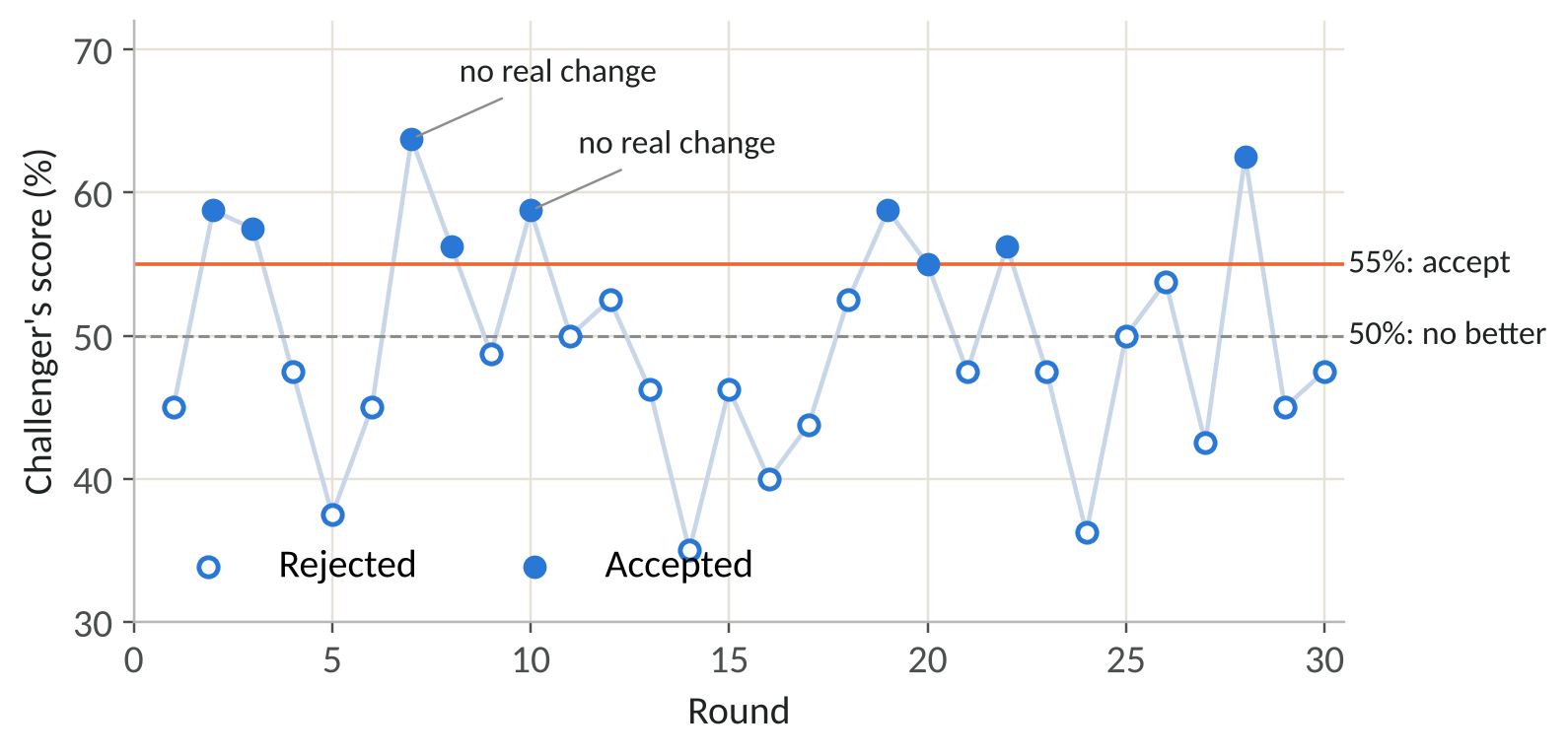
Figure 2: The challenger's score in each round of hill climbing. Rounds marked "no real change" altered a number by too little to change it after rounding.
Nine challengers were accepted. The learned numbers were the same as the originals except that advancing a man became worth 4 points instead of 3, and the centre became worth 2 instead of 4. In the final check, 200 games on new openings, the learned numbers scored 57.5% against the originals, with a 95% range from 50.6% to 64.4%.
That looks like success. Module 4 explains why we should not believe it yet.
Check your progress
Your run prints the same rounds and the same final check, because every random choice comes from a fixed seed. If your numbers differ slightly, check that your files match the listings.
Module 4: How Many Games Prove an Improvement?
The rounds that changed nothing
Look at the two rounds marked "no real change" in Figure 2. In round 7, the mutation tried to change the advance value from 4, but after rounding to a whole number it was still 4: the challenger was identical to the champion. It scored 63.7% and was accepted. In round 10 the same thing happened to the centre value, and the identical challenger scored 58.8%. Three more rounds with no real change scored 43.8%, 53.8% and 45.0%.
So two copies of the same program, playing 40 games, scored anywhere between 43.8% and 63.7%. That is pure luck, and it is bigger than most of the improvements the hill climbing was trying to find.
Putting a number on luck
Using the formula from Module 2, a 40-game match between equal players has a standard error of about 7.9 percentage points. Its 95% range is therefore about 50% plus or minus 15.5 points. Our acceptance bar of 55% is less than one standard error above 50%, so many accepted changes were probably accepted by luck. With 200 games the 95% range shrinks to about plus or minus 6.9 points, which is why the final checks use 200 games.
The independent check
The final check in Module 3 used a different set of openings from training, which is good practice. But we chose to stop and report after seeing it. To be sure, we ran a separate comparison with train/compare.js (Module 8), on yet another set of openings.
| Search depth | Learned numbers against the originals, 200 games |
|---|---|
| 3 (the training depth) | 53.5% (95% range 46.6% to 60.4%) |
| 4 | 53.5% (95% range 46.6% to 60.4%) |
Both ranges include 50%. The honest conclusion is that hill climbing may have found a small improvement, but our evidence is not strong enough to say so. The two results being identical is a coincidence of these particular games.
What to take from this
A small sample can make an identical program look much better or much worse
Always judge the final result on games that played no part in choosing it
Decide the size of the final test before you run it, and report it whatever it says
If you want stronger evidence, play more games. To halve the width of the 95% range you need four times as many
Teacher's note: This is the module to reread. Almost every exaggerated claim about AI, in business as well as in research, comes from skipping the steps above.
Module 5: A Maths Primer for Neural Networks
You do not need advanced maths for this course, but four ideas will make Modules 6 to 8 much easier.
1. A weighted sum
A single artificial neuron takes several numbers, multiplies each by its own weight, adds them up, and adds one more number called a bias. Our hand-written evaluation is already a weighted sum: so many men times 100, plus so many kings times 175, and so on.
2. Layers and activation functions
A neural network stacks neurons in layers. Our network has three.
An input layer of 128 numbers describing the position
A hidden layer of 32 neurons, each a weighted sum of all 128 inputs
An output layer of one neuron, a weighted sum of the 32 hidden values
Between layers, each value passes through an activation function. The hidden layer uses ReLU, which simply turns negative numbers into 0. That small bend is what lets the network learn patterns that are more than a straight sum. The output uses tanh, which squeezes any number into the range from -1 to +1, so the output reads as "expect to lose" at -1 up to "expect to win" at +1.
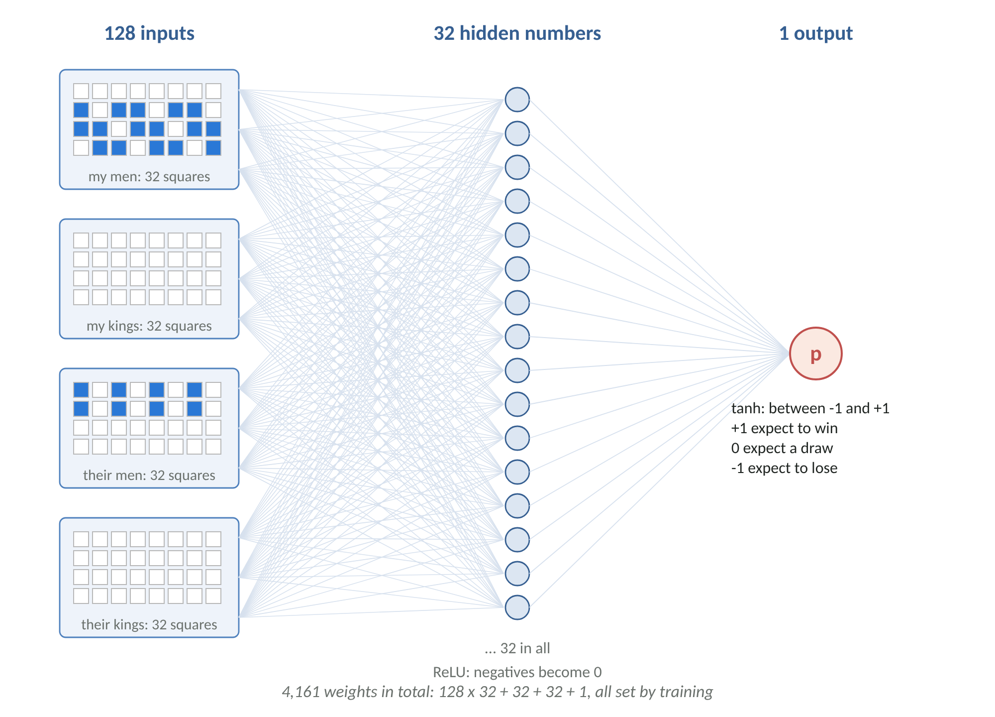
Figure 3: The network used in this course. Each line is a weight. Only some hidden neurons and lines are drawn.
3. Loss: measuring how wrong
To train the network we show it positions whose outcome we know, and compare its guess with the truth. The loss turns that comparison into one number. We use the mean squared error: for each position, take the guess minus the true result, square it, and average over all positions. Lower is better, and a perfect network would score 0.
4. Gradient descent: walking downhill
Training means finding weights that make the loss small. Picture the loss as the height of a landscape, with one direction for every weight. The gradient says which way is uphill and how steeply. Gradient descent repeatedly takes a small step the opposite way, downhill. The size of the step is the learning rate.
The gradient is worked out by backpropagation: starting from the loss, we use the chain rule from calculus to pass the blame backwards through each layer to each weight. You will see it written out in a few lines of Python in Module 7, and a test that checks it is right.
We use a popular refinement of gradient descent called Adam, which keeps a running average of recent gradients so that the steps are steadier.
Module 6: Making Training Data by Self-Play
Describing a position to the network
A network only understands numbers, so each position becomes 128 numbers, each 0 or 1. There are 32 dark squares, and four questions about each: is there one of my men here, one of my kings, one of their men, one of their kings? Four questions times 32 squares gives 128.
The position is always described from the point of view of the side to move. For White, the board is turned round, so "my pieces" always start at the bottom and move up. This way the network learns one set of patterns that works for both colours, instead of having to learn everything twice.
Create static/js/nn.js. It contains the description of the position, encode, and the calculation that runs the trained network, predict. It reads its weights from nn-weights.js, which Module 7 creates.
File: static/js/nn.js
/*
 * nn.js - a small neural network that judges draughts positions (Course 3).
 *
 * The network was trained in Python (train/train_nn.py) on positions from
 * self-play games. Its trained numbers are stored in nn-weights.js. This file
 * only does two things:
 *
 *   encode(board, player)   turn a position into 128 numbers (0 or 1)
 *   evaluate(board, player) run the network and return a score
 *
 * The encoding is always from the point of view of `player`: the board is
 * turned round for White, so "my pieces" always start at the bottom and move
 * up. The 128 inputs are four groups of 32, one number per dark square:
 *   0-31   my men        32-63  my kings
 *   64-95  their men     96-127 their kings
 */

const NeuralEval = (function () {
  const W = (typeof NN_WEIGHTS !== 'undefined') ? NN_WEIGHTS : require('./nn-weights.js');

  function encode(board, player) {
    const x = new Array(128).fill(0);
    let i = 0;
    for (let r = 0; r < 8; r++) {
      for (let c = 0; c < 8; c++) {
        if ((r + c) % 2 === 0) continue;               // light squares are never used
        // White sees the board turned round, so square i means the same to both.
        const p = player === 'b' ? board[r][c] : board[7 - r][7 - c];
        if (p !== '.') {
          const mine = (p.toLowerCase() === player);
          const king = (p === 'B' || p === 'W');
          x[(mine ? 0 : 64) + (king ? 32 : 0) + i] = 1;
        }
        i++;
      }
    }
    return x;
  }

  // Run the network: 128 inputs -> hidden layer (ReLU) -> 1 output (tanh).
  // The output is between -1 (expect to lose) and +1 (expect to win).
  function predict(board, player) {
    const x = encode(board, player);
    let out = W.b2;
    for (let h = 0; h < W.b1.length; h++) {
      let sum = W.b1[h];
      const row = W.W1[h];
      for (let k = 0; k < 128; k++) if (x[k]) sum += row[k];   // inputs are 0 or 1
      if (sum > 0) out += W.W2[h] * sum;                       // ReLU: ignore negatives
    }
    return Math.tanh(out);
  }

  // Minimax needs whole numbers on a scale like the hand-written rule.
  function evaluate(board, player) {
    return Math.round(1000 * predict(board, player));
  }

  return { encode, predict, evaluate };
})();

if (typeof module !== 'undefined') module.exports = NeuralEval;
Self-play
To learn which positions tend to be won, the network needs examples. train/selfplay.js makes the computer play itself 3,000 times, using a fast search of depth 2 with a few random moves for variety. For every position in every game, it records the 128 numbers and how that game finally ended for the side to move: +1 for a win, 0 for a draw and -1 for a loss.
File: train/selfplay.js
/*
 * train/selfplay.js - create training data for the neural network.
 *
 * The program plays itself many times. For every position in every game we
 * write down two things:
 *   x - the position, as the 128 numbers the network reads (see nn.js)
 *   y - how the game finally ended for the side to move: +1 won, 0 draw, -1 lost
 * The network will learn to look at x and guess y. In other words, it learns
 * "positions like this one tend to be won".
 *
 * Run:  node train/selfplay.js [games]
 * Writes train/data/positions.jsonl, one position per line.
 */

const fs = require('fs');
const path = require('path');
const NeuralEval = require('../static/js/nn.js');
const { seeded, randomOpening, playGame } = require('./match.js');

const GAMES = Number(process.argv[2] || 3000);
// Shallow search with a little randomness: fast, and varied enough to learn from.
const PLAYER = { depth: 2, randomChance: 0.1, evaluator: 'hand' };

const rand = seeded(42);
const out = fs.createWriteStream(path.join(path.dirname(__filename), 'data', 'positions.jsonl'));
const totals = { b: 0, w: 0, draw: 0 };
let positions = 0;

for (let game = 0; game < GAMES; game++) {
  const seen = [];
  const winner = playGame(randomOpening(rand), PLAYER, PLAYER, rand, 200,
                          state => seen.push(state));
  totals[winner]++;
  for (const state of seen) {
    const y = winner === 'draw' ? 0 : (winner === state.turn ? 1 : -1);
    const x = NeuralEval.encode(state.board, state.turn).join('');
    out.write(JSON.stringify({ game, x, y }) + '\n');
    positions++;
  }
  if ((game + 1) % 500 === 0) console.log(`${game + 1} games, ${positions} positions`);
}
out.end();
console.log('Results:', totals, 'Positions written:', positions);
node train/selfplay.js 3000
On the computer used for this course, the 3,000 games ended with 1,148 wins for Black, 1,154 for White and 698 draws, and produced 401,043 positions. The file train/data/positions.jsonl is about 60 MB, which is why it stays on your computer and is never copied to the server.
Teacher's note: Our labels are noisy. A position early in a game is labelled with a result that depends on many later moves, some of them random. The network has to find the signal under that noise, and that is one reason it struggles in Module 8.
Module 7: Training the Network in Python
Training, validation and baselines
The script holds back ten per cent of the games for validation. The network never trains on them, so the validation loss shows how well it copes with positions it has not seen. We split by game, not by position, because positions from the same game are very alike: testing on them would flatter the network.
Before training, the script also measures two baselines, simple rules the network must beat to have learned anything worth having: always guessing 0, and counting the pieces.
The listing
Create train/train_nn.py. Every step of Module 5 is here: forward, loss, gradients and the Adam update in main.
File: train/train_nn.py
"""
train/train_nn.py - train a small neural network to judge draughts positions.

The network is written by hand with NumPy, so every step is visible:

    inputs x (128 numbers, 0 or 1)
      -> hidden layer: h = relu(W1 . x + b1)      (HIDDEN numbers)
      -> output:       p = tanh(W2 . h + b2)      (one number, -1 to +1)

Training repeats four steps on small batches of positions:
    1. FORWARD   - work out p for each position
    2. LOSS      - measure how wrong p is: mean of (p - y) squared
    3. BACKWARD  - work out how each weight affected the loss (the gradient)
    4. UPDATE    - nudge every weight a little in the direction that lowers the loss

Ten per cent of the GAMES are held back for validation. The network never
trains on them, so the validation loss shows how well it handles positions it
has not seen. Splitting by game, not by position, matters: positions from the
same game are very alike, and testing on them would flatter the network.

Run:  python train/train_nn.py
Reads train/data/positions.jsonl, writes static/js/nn-weights.js
"""

import json
import os

import numpy as np

HERE = os.path.dirname(os.path.abspath(__file__))
HIDDEN = 32
EPOCHS = 15
BATCH = 256
LEARNING_RATE = 0.001
rng = np.random.default_rng(1)


def load():
    xs, ys, games = [], [], []
    with open(os.path.join(HERE, "data", "positions.jsonl")) as f:
        for line in f:
            row = json.loads(line)
            xs.append(np.frombuffer(row["x"].encode(), dtype=np.uint8) - 48)   # "0101" -> [0,1,0,1]
            ys.append(row["y"])
            games.append(row["game"])
    return (np.array(xs, dtype=np.float32), np.array(ys, dtype=np.float32),
            np.array(games))


def baselines(x_train, y_train, x_val, y_val):
    """Simple rules the network must beat, or it has learned nothing useful."""
    print(f"  baseline 'always guess 0' : {np.mean(y_val ** 2):.4f}")
    # Piece count: my pieces minus theirs, kings counted as 1.5, squashed with tanh.
    def material(x):
        return x[:, 0:32].sum(1) + 1.5 * x[:, 32:64].sum(1) - x[:, 64:96].sum(1) - 1.5 * x[:, 96:128].sum(1)
    best = min((np.mean((np.tanh(k * material(x_train)) - y_train) ** 2), k)
               for k in np.linspace(0.05, 1.0, 20))
    k = best[1]
    print(f"  baseline 'count the pieces': {np.mean((np.tanh(k * material(x_val)) - y_val) ** 2):.4f}")


def forward(params, xb):
    """1. FORWARD: inputs -> hidden layer -> prediction between -1 and +1."""
    W1, b1, W2, b2 = params
    z = xb @ W1.T + b1
    h = np.maximum(z, 0)                  # ReLU: negative values become 0
    p = np.tanh(h @ W2 + b2)
    return z, h, p


def loss(params, xb, yb):
    """2. LOSS: the average squared error."""
    return float(np.mean((forward(params, xb)[2] - yb) ** 2))


def gradients(params, xb, yb):
    """3. BACKWARD: how much the loss changes as each weight changes (the chain rule)."""
    W1, b1, W2, b2 = params
    z, h, p = forward(params, xb)
    d_out = 2 * (p - yb) / len(yb) * (1 - p ** 2)     # back through the loss and tanh
    gW2 = h.T @ d_out
    gb2 = d_out.sum()
    d_h = np.outer(d_out, W2) * (z > 0)               # back through ReLU
    gW1 = d_h.T @ xb
    gb1 = d_h.sum(0)
    return [gW1, gb1, gW2, gb2]


def main():
    x, y, games = load()
    is_val = games % 10 == 0
    x_train, y_train, x_val, y_val = x[~is_val], y[~is_val], x[is_val], y[is_val]
    print(f"{len(y_train)} training positions, {len(y_val)} validation positions")
    print("Validation loss of simple rules (lower is better):")
    baselines(x_train, y_train, x_val, y_val)

    # Start with small random weights.
    params = [rng.normal(0, 0.1, (HIDDEN, 128)).astype(np.float32),   # W1
              np.zeros(HIDDEN, np.float32),                           # b1
              rng.normal(0, 0.1, HIDDEN).astype(np.float32),          # W2
              np.float32(0)]                                          # b2
    # Adam keeps a running average of each gradient (m) and of its square (v),
    # which makes the steps steadier than plain gradient descent.
    m = [np.zeros_like(p) for p in params]
    v = [np.zeros_like(p) for p in params]
    step = 0

    best_val, best_params = None, None
    for epoch in range(1, EPOCHS + 1):
        order = rng.permutation(len(y_train))
        for start in range(0, len(order), BATCH):
            idx = order[start:start + BATCH]
            grads = gradients(params, x_train[idx], y_train[idx])
            step += 1                                       # 4. UPDATE (Adam)
            for i, g in enumerate(grads):
                m[i] = 0.9 * m[i] + 0.1 * g
                v[i] = 0.999 * v[i] + 0.001 * g ** 2
                m_hat = m[i] / (1 - 0.9 ** step)
                v_hat = v[i] / (1 - 0.999 ** step)
                params[i] = params[i] - LEARNING_RATE * m_hat / (np.sqrt(v_hat) + 1e-8)
        train_loss = loss(params, x_train, y_train)
        val_loss = loss(params, x_val, y_val)
        print(f"epoch {epoch:2d}: training loss {train_loss:.4f}, validation loss {val_loss:.4f}")
        # Keep the version that did best on validation, in case later epochs overfit.
        if best_val is None or val_loss < best_val:
            best_val = val_loss
            best_params = [np.copy(p) for p in params]

    W1, b1, W2, b2 = best_params
    weights = {"hidden": HIDDEN, "W1": np.round(W1.astype(float), 5).tolist(),
               "b1": np.round(b1.astype(float), 5).tolist(),
               "W2": np.round(W2.astype(float), 5).tolist(), "b2": round(float(b2), 5),
               "validation_loss": round(float(best_val), 4)}
    out = os.path.join(HERE, "..", "static", "js", "nn-weights.js")
    with open(out, "w") as f:
        f.write("// nn-weights.js - written by train/train_nn.py. Do not edit by hand.\n")
        f.write(f"// Best validation loss: {best_val:.4f}\n")
        f.write("const NN_WEIGHTS = " + json.dumps(weights) + ";\n")
        f.write("if (typeof module !== 'undefined') module.exports = NN_WEIGHTS;\n")
    print(f"Saved the best network (validation loss {best_val:.4f}) to {os.path.normpath(out)}")


if __name__ == "__main__":
    main()
python train/train_nn.py
What happened
Figure 4 shows the training run made for this course.
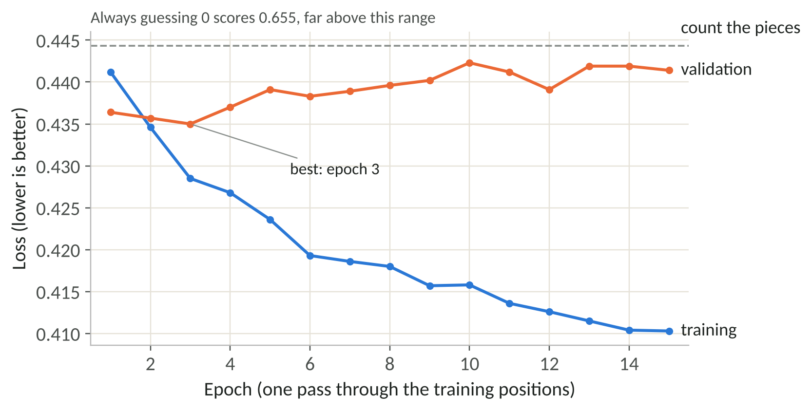
Figure 4: Training and validation loss in each epoch, with the piece-counting baseline.
Always guessing 0 gave a validation loss of 0.6547, and counting the pieces 0.4443. The network did best on validation after three epochs, at 0.4350: better than counting the pieces, but only a little. After that, the training loss kept falling while the validation loss rose. The network was starting to memorise the training games instead of learning patterns that carry over to new ones. This is called overfitting, and it is why the script keeps the version that did best on validation, not the last one. Stopping at the best validation result is called early stopping.
Checking the maths
Backpropagation written by hand is easy to get subtly wrong, and a wrong gradient often still trains, just badly. The classic check is to nudge one weight by a tiny amount, measure how much the loss really changes, and compare that with what the gradient predicted. tests/test_learn.py does exactly that, and is listed in Module 9.
Module 8: Running the Network inside Minimax
Three ways to use the network
The network's output is between -1 and +1. Minimax needs whole numbers on a similar scale to the hand-written rule, so NeuralEval.evaluate multiplies by 1,000 and rounds.
We compared three evaluations against the hand-written rule.
Learned numbers: the result of Module 3
Neural network alone: the network replaces the rule completely
Hybrid: the hand-written rule, plus 300 times the network's output. The rule supplies solid knowledge, and the network nudges it where it has learned something the rule misses. The 300, about three men, was a first guess and was not tuned
The comparison
train/compare.js plays each against the hand-written rule, at the same depth, on openings used nowhere else.
File: train/compare.js
/*
 * train/compare.js - the final exam: does a learned evaluation actually play better?
 *
 * Each contender plays the hand-written evaluation from Course 1 with the SAME
 * search depth, on openings never used in training. Only the judgement of
 * positions differs, so any difference in score comes from the evaluation.
 *
 * Run:  node train/compare.js [depth] [pairs]
 */

const { match, describe } = require('./match.js');

const DEPTH = Number(process.argv[2] || 4);
const PAIRS = Number(process.argv[3] || 50);
const at = evaluator => ({ depth: DEPTH, randomChance: 0, evaluator });

console.log(`Search depth ${DEPTH}, ${PAIRS * 2} games each, against the hand-written evaluation:`);
for (const name of ['learned', 'neural', 'hybrid']) {
  const started = Date.now();
  const r = match(at(name), at('hand'), PAIRS, 424242);
  console.log(`  ${name.padEnd(8)} ${describe(r)}  [${((Date.now() - started) / 1000).toFixed(0)} s]`);
}
node train/compare.js 3 100
node train/compare.js 4 100
Figure 5 shows the results.
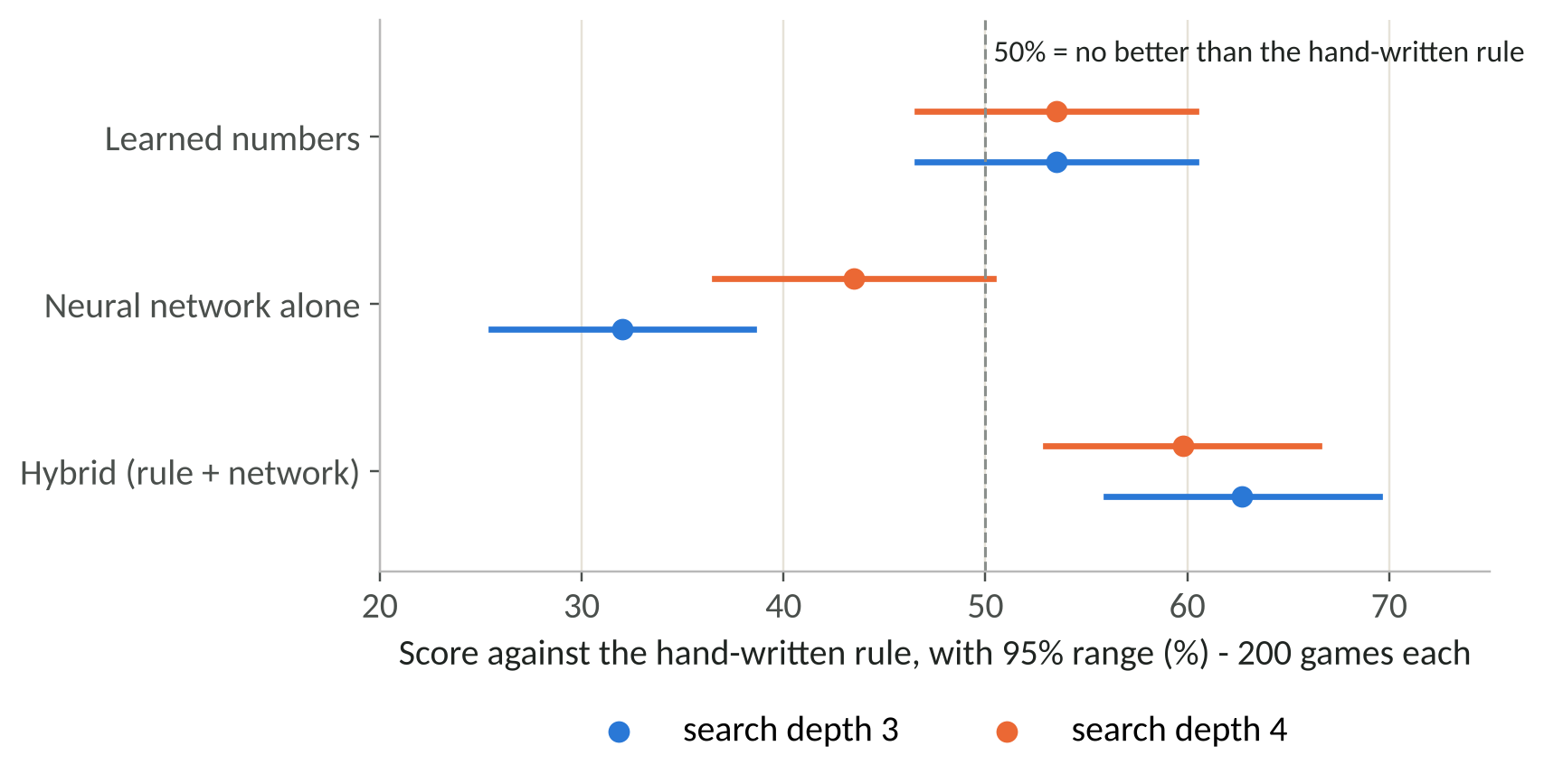
Figure 5: Each learned evaluation's score against the hand-written rule, with 95% ranges, at search depths 3 and 4.
| Evaluation | Depth 3, 200 games | Depth 4, 200 games |
|---|---|---|
| Learned numbers | 53.5% (46.6% to 60.4%) | 53.5% (46.6% to 60.4%) |
| Neural network alone | 32.0% (25.5% to 38.5%) | 43.5% (36.6% to 50.4%) |
| Hybrid | 62.7% (56.0% to 69.5%) | 59.8% (53.0% to 66.5%) |
What the results mean
The network on its own plays clearly worse than the hand-written rule, even though it predicted results slightly better than counting the pieces. Predicting who will win from a position, on average, is not the same skill as telling apart two similar positions at the end of a search. The network learned from weak, noisy games, and its judgement is too coarse for that second job.
The hybrid is the clear success. At both depths its whole 95% range lies above 50%. Combining human knowledge with a learned correction did better than either the rule or the network alone. This combination is common in real systems: learning works best when it builds on what is already known.
Adding the new levels to the game
The LEVELS table in ai.js already contains the two new levels: Learned searches to depth 7 like High, and Neural uses the hybrid evaluation at depth 5, because each evaluation takes longer. On the computer used for this course, Neural took a median of 31 milliseconds per move and at most 71, and Learned a median of 91 and at most 314. Add the two options to the setup dialog and load the new scripts before ai.js.
From static/index.html
        <label><input type="radio" name="level" value="hard"> High</label>
        <label><input type="radio" name="level" value="learned"> Learned</label>
        <label><input type="radio" name="level" value="neural"> Neural</label>
From static/index.html
  <script src="js/rules.js"></script>
  <!-- Course 3: the learned numbers and the neural network load before the AI. -->
  <script src="js/learned-weights.js"></script>
  <script src="js/nn-weights.js"></script>
  <script src="js/nn.js"></script>
Finally, give the new levels names in main.js, so the scoreboard shows "Computer (Learned)" and "Computer (Neural)".
From static/js/main.js
const LEVEL_NAMES = { easy: 'Low', medium: 'Medium', hard: 'High',
                      learned: 'Learned', neural: 'Neural' };
Check your progress
Both new levels appear in the setup dialog and play legal moves, and your comparison results match the table above.
Module 9: Testing
The JavaScript tests check that mirror-image positions look the same to the network, that each evaluation returns whole numbers, that every level plays a legal move, and that identical players score close to 50%.
File: tests/test_learn.js
// Run with:  node tests/test_learn.js
// Checks the parts of Course 3 that run in JavaScript.
const test = require('node:test');
const assert = require('node:assert');
const Rules = require('../static/js/rules.js');
const AI = require('../static/js/ai.js');
const NeuralEval = require('../static/js/nn.js');
const { match } = require('../train/match.js');

// Turn a position round and swap the colours: the mirror image for the other player.
function mirror(board) {
  const swap = { b: 'w', w: 'b', B: 'W', W: 'B', '.': '.' };
  return board.map((row, r) => row.map((_, c) => swap[board[7 - r][7 - c]]));
}

test('the network sees mirror-image positions the same way', () => {
  let state = Rules.newGame();
  for (let i = 0; i < 6; i++) state = Rules.applyMove(state, Rules.legalMoves(state)[0]);
  const asBlack = NeuralEval.encode(state.board, 'b');
  const asWhiteInMirror = NeuralEval.encode(mirror(state.board), 'w');
  assert.deepStrictEqual(asBlack, asWhiteInMirror);
});

test('the encoding has one input per piece', () => {
  const x = NeuralEval.encode(Rules.newGame().board, 'b');
  assert.strictEqual(x.length, 128);
  assert.strictEqual(x.reduce((a, b) => a + b, 0), 24);
});

test('every evaluator returns whole numbers', () => {
  const board = Rules.newGame().board;
  assert.ok(Number.isInteger(AI.evaluateWith(AI.WEIGHTS, board, 'b')));
  assert.ok(Number.isInteger(NeuralEval.evaluate(board, 'b')));
});

test('every level, old and new, returns a legal move', () => {
  const state = Rules.newGame();
  const legal = Rules.legalMoves(state).map(m => JSON.stringify(m.path));
  for (const level of Object.keys(AI.LEVELS)) {
    assert.ok(legal.includes(JSON.stringify(AI.chooseMove(state, level).path)), level);
  }
});

test('a match between identical players is close to even', () => {
  const same = { depth: 2, randomChance: 0, evaluator: 'hand' };
  const r = match(same, same, 20, 5);
  assert.ok(r.low <= 0.5 && r.high >= 0.5, `score ${r.score}`);
});
The Python tests check the gradients against a numerical estimate, as described in Module 7, and that the output always lies between -1 and +1.
File: tests/test_learn.py
"""Run with:  python tests/test_learn.py   (needs NumPy)"""
import os
import sys

import numpy as np

sys.path.insert(0, os.path.join(os.path.dirname(os.path.dirname(os.path.abspath(__file__))), "train"))
import train_nn  # noqa: E402


def test_gradients_match_a_numerical_estimate():
    """
    The classic check for hand-written backpropagation: nudge one weight a
    tiny amount, see how much the loss really changes, and compare with the
    gradient our formula predicts. They should agree closely.
    """
    rng = np.random.default_rng(0)
    params = [rng.normal(0, 0.5, (4, 128)), rng.normal(0, 0.1, 4), rng.normal(0, 0.5, 4), 0.1]
    x = (rng.random((8, 128)) < 0.2).astype(float)
    y = rng.choice([-1.0, 0.0, 1.0], 8)
    grads = train_nn.gradients(params, x, y)
    eps = 1e-6
    for (i, index) in [(0, (1, 5)), (1, (2,)), (2, (3,))]:
        bumped = [np.array(p, dtype=float) for p in params]
        bumped[i][index] += eps
        numeric = (train_nn.loss(bumped, x, y) - train_nn.loss(params, x, y)) / eps
        assert abs(numeric - grads[i][index]) < 1e-4, (i, numeric, grads[i][index])


def test_prediction_is_between_minus_one_and_one():
    rng = np.random.default_rng(1)
    params = [rng.normal(0, 3, (4, 128)), np.zeros(4), rng.normal(0, 3, 4), 0.0]   # large weights
    p = train_nn.forward(params, (rng.random((20, 128)) < 0.3).astype(float))[2]
    assert np.all(p >= -1) and np.all(p <= 1)


if __name__ == "__main__":
    for name, fn in list(globals().items()):
        if name.startswith("test_"):
            fn()
            print("passed", name)
node tests/test_rules.js
node tests/test_learn.js
python tests/test_learn.py
Check your progress
All the tests pass: 8 and 5 tests in the JavaScript files, and two lines starting with passed from the Python file.
Module 10: Deploying the Learned Levels
Nothing new needs installing on the server: the learning happened on your computer, and the results are four small JavaScript files. Copy the changed static files to the server as in Course 1, Module 11.
scp -r static you@your-server:/var/www/draughts/Do not copy the train folder. It holds 60 MB of training data and tools the server never uses.
Open the game in a browser, choose Neural, and play a game. If the page loads but the computer never moves, open the browser's developer tools (F12) and look at the Console: the most likely cause is a script loading in the wrong order in index.html.
Teacher's note: The game ran with these files on Ubuntu 24.04 with Apache2 in the Course 1 set-up. Nothing in this course changes the server side.
Module 11: Where to Go Next
Tune the hybrid. HYBRID_SCALE was a first guess. Try 150 and 600 with
compare.js, and keep a separate set of openings for the final checkTrain on better games. Generate self-play data at depth 4 instead of 2. The games will be slower but the labels less noisy
Hill-climb with more games. Use 100 games per round and a stricter acceptance bar, then check the result at depth 4
Learn from the search itself. Instead of the game's final result, train the network to predict the score of a deeper search from each position. This idea, learning from one's own later predictions, is behind much stronger game programs
Known limitations
Results depend on the seeds. Different openings give somewhat different numbers, which is why every result is quoted with its 95% range
The network is small and its data weak. It was chosen so that training takes seconds on a laptop, not to be as strong as possible
The 95% ranges are approximate. They use a simple formula that treats draws roughly
Glossary of Terms
| Term | Meaning |
|---|---|
| 95% range | The band in which the true value is expected to lie, 95 times in 100, given the luck in a sample |
| Activation function | A simple function applied to each neuron's value, such as ReLU or tanh, that lets a network learn curved patterns |
| Adam | A widely used improvement on gradient descent that keeps running averages of recent gradients |
| Backpropagation | Working out every weight's gradient by passing the error backwards through the network with the chain rule |
| Baseline | A simple method that a learned model must beat to show it has learned something useful |
| Bias | A number added to a neuron's weighted sum, adjusted in training like a weight |
| Early stopping | Keeping the version of a model that did best on validation data, before it began to overfit |
| Epoch | One complete pass through all the training data |
| Gradient | How much, and in which direction, the loss changes as each weight changes |
| Gradient descent | Training by repeatedly nudging every weight a little in the direction that lowers the loss |
| Hill climbing | Improving something by making small changes and keeping only those that help |
| Hybrid evaluation | The hand-written rule plus a correction from the neural network |
| Learning rate | How big each step of gradient descent is |
| Loss | A single number measuring how wrong a model's guesses are. Lower is better |
| Mean squared error | A loss: the average of the squared differences between guesses and true values |
| Neural network | A model made of layers of simple connected calculations whose weights are set by training |
| Neuron | One unit of a neural network: a weighted sum of its inputs plus a bias, passed through an activation function |
| NumPy | A Python package for fast calculations on large tables of numbers |
| Overfitting | When a model learns its training data too closely and does worse on new data |
| Parameter | A number in a program or model that can be set differently, by hand or by learning |
| ReLU | An activation function that turns negative numbers into 0 and leaves others unchanged |
| Seed | The starting value for a random number generator. The same seed always gives the same sequence |
| Self-play | A program playing against a copy of itself to produce results it can learn from |
| Standard error | A measure of how much a result would vary from sample to sample by luck alone |
| tanh | An activation function that squeezes any number into the range from -1 to +1 |
| Validation data | Data held back from training and used only to check how well a model copes with new examples |
| Weight | A number inside a model that multiplies one of its inputs, set by training |
Appendix: Sources
| Topic | Source |
|---|---|
| Course 1 | Building an AI Draughts Game for the Web, OUTPUTS/Draughts AI Course/ |
| Learning by self-play | Samuel, A. L. (1959) "Some Studies in Machine Learning Using the Game of Checkers", IBM Journal of Research and Development, 3(3), pp. 210-229: https://people.csail.mit.edu/brooks/idocs/Samuel.pdf |
| Backpropagation | Rumelhart, D. E., Hinton, G. E. and Williams, R. J. (1986) "Learning representations by back-propagating errors", Nature, 323, pp. 533-536 |
| Adam | Kingma, D. P. and Ba, J. (2014) "Adam: A Method for Stochastic Optimization": https://arxiv.org/abs/1412.6980 |
| NumPy | NumPy documentation: https://numpy.org/doc/stable/ |
| Results quoted in this course | The output files in the course's train/data folder: hillclimb-output.txt, hillclimb-log.json, train_nn-output.txt, compare-depth3.txt and compare-depth4.txt |
| Virtual environments cannot be copied | Python documentation, venv: https://docs.python.org/3/library/venv.html |
| AirPlay Receiver using port 5000 on a Mac | Apple Developer Forums, Why is Control Center on Monterey listening on ports?: https://developer.apple.com/forums/thread/682332 |